
Data Parallelism: Scaling LLM Training Through Parallel Processing

In my latest article , I discussed the theoretical memory usage needed for inference and training with LLMs, highlighting the memory cost of each component involved in the process. Luckily for us, there exist many techniques that allow us to scale to larger models, heavily reducing the memory requirements that are only theoretical. Therefore, I want to start this series about parallelization and how it affects both inference and training workflows. We will start from the most basic approach, called Data Parallelism.
The anatomy of Data Parallelism

Have you ever found yourself in line at a supermarket and asked yourself “why the hell are they not opening other registers?” Maybe I’m the only one, but I find myself asking that question quite often, and each time I think that paying for your groceries is an embarrassingly parallel operation. That means that the process of me handing my groceries to the person at the register, them scanning the items, and me paying is a set of operations that are completely disconnected and unrelated from other people doing the same. There’s no dependency between people paying for their groceries and me doing the same. In computer science, this is called embarrassingly parallel, and it’s very nice when an algorithm has this property because it means that it can be parallelized quite easily. For example, if you have an algorithm that decreases each pixel value in an image by 1, you could technically use as many threads as there are pixels in the image, with each thread working independently and in parallel with the others.
The idea of Data Parallelism is essentially the same. Imagine you’re training a model and you have 8 GPUs at your disposal. For simplicity, let’s assume that you’re able to train your model on a single GPU. What do you do with the other 7? Well, you could instantiate 7 additional replicas of your model, each one hosted on a separate GPU. Then, you could train all the replicas in parallel. However, things aren’t quite that straightforward.
Understanding the Fundamentals: World Size, Batch Sizes, and Ranks
Let’s start from the usual scenario: we have a model θ and a dataset D. At each iteration, we sample a batch of data from the dataset D, and the number of samples in each batch we call the batch size. Let’s change this name and call it the global batch size, because this quantity indicates how many samples are being processed per step in our world. Our world is the totality of parallel processes that are involved. So, in practice for our example, the world size is also the number of GPUs we have at our disposal, since each GPU will run a parallel process.
If we have a global batch size, we also must have a local batch size, which represents how many samples each rank (or GPU) processes at a given step. This is typically called the micro batch size (mbs). In our case of Data Parallelism, it’s quite straightforward to determine what the micro batch size will be. It’s simply the global batch size divided by the number of model replicas, which in our case is 8.
For simplicity, we use dp to refer to the dimension of the Data Parallel setup.
The picture below helps visualizing how the global batch, denoted as bs is split into bs/N micro-batch sizes, called mbs:
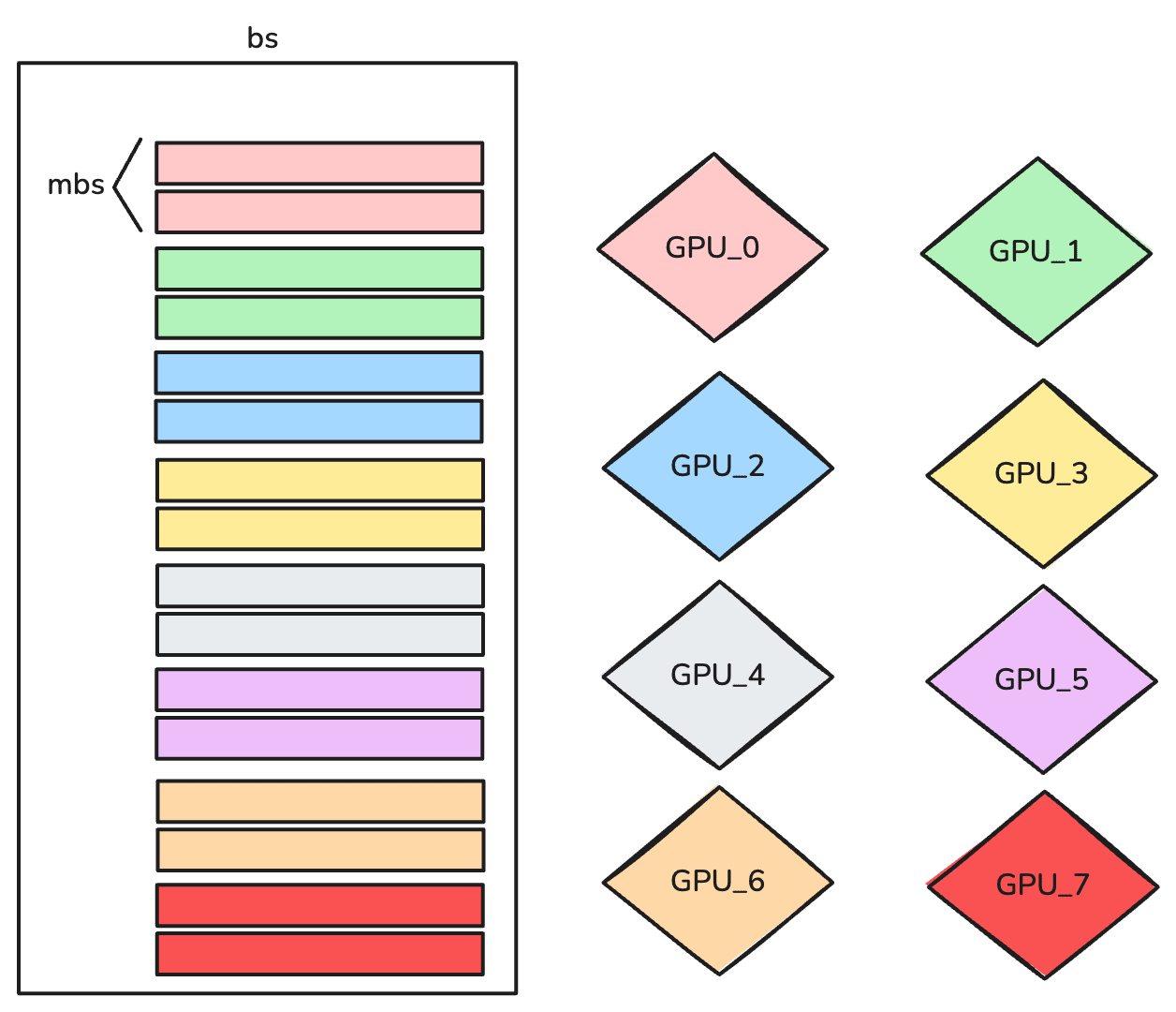
In this case, our global batch size is 16, however each GPU will process a local batch size of 2.
The Synchronization Challenge
However, if each GPU, which in our case hosts a model replica, performs the usual training of the model locally, we will end up with 8 different models, since each one has been trained on different data. And we really don’t want that. Therefore, we have to synchronize the training among all ranks, such that we keep the replicas identical across all GPUs. That’s not particularly difficult to achieve.
Here’s how the synchronization works: First, each GPU processes its local batch, computing the gradients for it. Then, we average all gradients and provide the result to each rank, such that each replica can be updated in the same way. This operation is called an All-Reduce. Think of it as a coordinated procedure where each specialist (GPU) performs their analysis (gradient computation) independently, and then all findings are shared and averaged to ensure every team member has the same complete picture before proceeding with the treatment (parameter update).
Here’s a visualization to help you understand this operation:
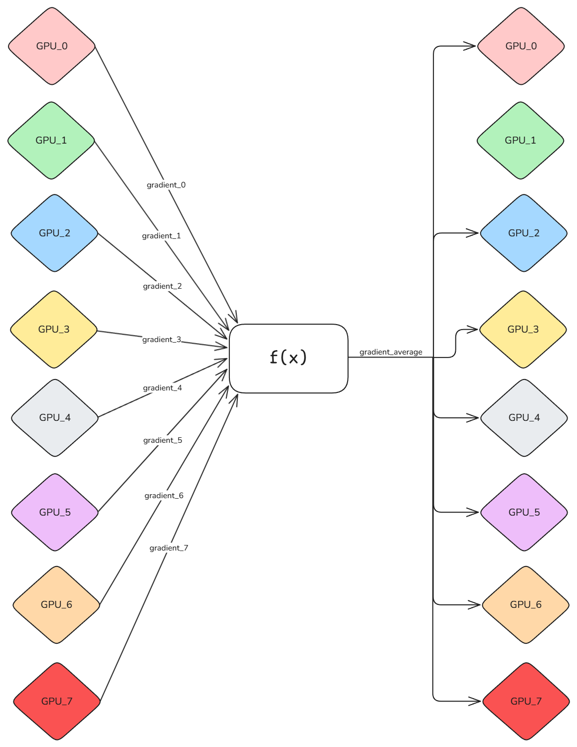
By definition, the All-Reduce operation can perform any operation f(x), and in our case we consider it to be the average. Once all the ranks receive the average of the gradients, the optimizer step can be performed on each replica, keeping them consistent across all ranks
To put in math what we’ve described so far, we can say that in data parallelism, we maintain identical copies of the model parameters θ across N devices. Each device processes a different subset of the training batch, computing local gradients that must be aggregated before updating the global parameters.
For a loss function L(θ, x, y) and a global batch B partitioned into N local sub-batches {B₁, B₂, ..., Bₙ}, each device i computes:
while the global gradient becomes:
The Sequential Trap
Now, if you’re thinking “Great! Problem solved, let’s just implement this and call it a day,” hold on a second. I don’t know about you, but suddenly I feel an overwhelming presence. It’s like a heavy weight on my chest, I can feel its pressure. Looking into the distance, I see him! It’s the machine learning optimization raccoon god! He’s repeating his mantra:

Of course! How could we have missed it! We fell into a sequentiality trap!
Picture this timeline: each GPU crunches through its local batch, computing gradients. Then, everything stops. All GPUs wait while the All-Reduce operation shuffles gradients around the network. Only after this communication dance completes can the optimizer finally update the parameters.
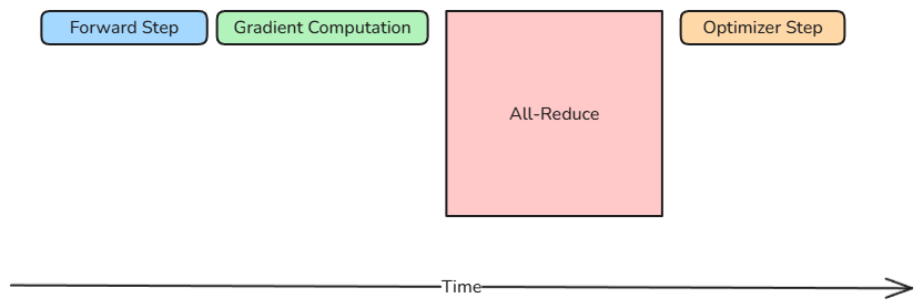
Do you see the problem? During that entire All-Reduce block, your expensive GPUs are sitting idle, twiddling their metaphorical thumbs. It’s like having a team of surgeons standing around waiting for test results when they could be preparing for the next procedure. Pure waste.
This sequential approach creates a bottleneck that gets worse as you add more GPUs or increase model size. The bigger your model, the more gradients to communicate. The more GPUs you have, the more complex the All-Reduce becomes. Something has to give.
The Gradient Pipeline
Here’s where understanding the backward pass becomes your secret weapon. When neural networks compute gradients, they work backwards through the layers using the chain rule. This isn’t just a mathematical quirk, it’s an opportunity.
Think about it: to compute the gradient for the final layer, you only need the model’s output. But for the second-to-last layer, you first need the final layer’s gradient. This creates a natural dependency chain that flows backward through your network.
The clever insight? We can start communicating gradients as soon as they’re computed, layer by layer. While the All-Reduce is busy shuffling the final layer’s gradients across the network, your GPU can already be computing gradients for the previous layer. No more waiting around.
Here’s what this overlapped approach looks like:
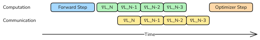
The green blocks show gradient computation for each layer, while the yellow blocks represent the communication happening in parallel. Notice how computation and communication now dance together instead of stepping on each other’s toes.
This technique, often called gradient bucketing, can dramatically reduce the effective communication overhead. Instead of your GPUs sitting idle during All-Reduce, they’re staying busy with useful work.
The Network Reality Check
Now, before we get too excited about our elegant gradient pipelining solution, let’s talk about the elephant in the room: networking. Yes, the “boring” infrastructure stuff that us ML practitioners often try to ignore. But here’s the thing: networking can make or break your entire parallelization strategy.
Let’s ground this in our example. We’ve been assuming one model replica per GPU, which works beautifully when those GPUs live in the same node. Why? Because GPUs within the same machine are connected by blazingly fast interconnects like NVIDIA’s NVLink. We’re talking serious bandwidth here: the latest NVLink technology in GB300s can push 1800GB/s. Even “older” setups with 8 A100s using NVLink 3.0 can achieve 600GB/s between GPUs. That’s fast enough to make your All-Reduce operations feel almost instantaneous.
But reality has a way of humbling us. What happens when your model replicas span multiple nodes? Welcome to the world of inter-node networking, where things get significantly more constrained.
InfiniBand represents the current gold standard for high-performance computing clusters. At its best, you might see 400GB/s of bandwidth, which is impressive by networking standards, but notice how it’s already slower than even older NVLink versions. Many clusters run InfiniBand configurations that top out at 200GB/s or even 100GB/s. Suddenly, that All-Reduce operation that was lightning-fast within a node becomes the bottleneck for your entire training run.
If your cluster runs on Ethernet (and many do, especially in cloud environments), prepare for a more sobering experience. Even high-end Ethernet tops out around 10GB/s, nearly two orders of magnitude slower than what you get with NVLink. At these speeds, communication overhead can easily dominate your training time, making data parallelism feel more like “data crawling.”
This networking hierarchy creates a fundamental challenge for scaling. As you add more nodes to accommodate larger models or larger batch sizes, the communication bottleneck grows increasingly severe. It’s why networking has become one of the primary limiting factors for training the largest language models. The math is simple but brutal: if you spend more time moving data than computing, adding more GPUs doesn’t help, it just gives you more expensive paperweights.
Closing the Incision
Well, there you have it, our first surgical procedure in the parallelization operating room. Data parallelism might look simple from the outside, but as any good surgeon knows, even routine operations can have complications if you don’t understand the anatomy underneath.
We’ve successfully diagnosed the sequential bottleneck, performed some gradient pipelining surgery, and learned that networking can be the difference between a successful operation and a patient flatining on the table.
Next time, we’ll scrub in for model parallelism: what happens when your neural network patient is too big to fit on our operating table? Bring your scalpel, it’s going to get messy.
Until then, keep your gradients sharp and your All-Reduces faster than a cardiac surgeon’s hands!