Transformer Attention, Backwards

You already know what a language model does. Let's reverse-engineer how.

You type a prompt. The model spits out the next word. Then the next. Then the next.

But what actually happens inside? Everyone explains transformers front-to-back: embeddings, positional encodings, attention heads, feed-forward layers, output. That’s the anatomy textbook approach. Accurate, but it buries the why under a pile of what.

We’re going to do the opposite. We start from the end result and work backwards, like a surgeon who first studies the symptom, then traces it back to the organ that caused it.

The Diagnosis: it's just a classification problem

So let’s start at the very end. The model has processed your entire prompt and is about to produce the next token. What’s actually happening in that moment?

Here’s the punchline that nobody leads with: a language model, at its core, solves a classification problem.

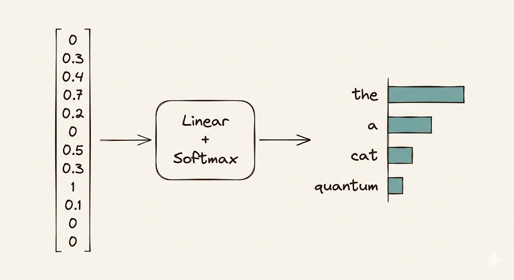
The model has a vocabulary of, say, 50,000 tokens. At every single generation step, its job is to look at a vector (the hidden state of the last token in the sequence) and decide: which of these 50,000 tokens comes next?

That’s it. A single vector goes into a linear layer, out comes a score for each token in the vocabulary, softmax turns those scores into probabilities, and the highest one wins (or gets sampled from, depending on your temperature settings).

So the real question becomes: what does that final vector need to contain for this classification to work well?

The Clinical Summary: one vector to rule them all

Ok so we know the endgame: classify one vector into one of 50,000 tokens. That immediately raises the stakes for what that vector actually contains. If it’s garbage, the prediction is garbage. If it’s good, it needs to be really good.

Think of it like a clinical summary before surgery. You don’t re-read the patient’s entire file in the operating room. You need a single, dense document that captures everything relevant: history, current symptoms, allergies, risk factors. Miss one detail and you cut the wrong thing.

That final hidden-state vector is the model’s clinical summary of the entire input sequence. It needs to encode:

• What the sentence is about (semantics)

• The grammatical structure so far (syntax)

• Which entities were mentioned and how they relate to each other

• The tone, the context, the subtle cues that determine what word logically follows

All of that, compressed into a single vector of (typically) a few thousand dimensions.

Now the question shifts: how does the model build such a rich representation from a sequence of tokens?

The Presenting Symptom: words in isolation are meaningless

So we need a great summary vector, built from the input tokens. The naive approach would be to just process each token independently and hope for the best. But that falls apart almost immediately.

Words don’t mean anything in isolation. “Bank” means one thing after “river” and another after “savings.” “It” could refer to anything. “Light” could be a noun, adjective, or verb.

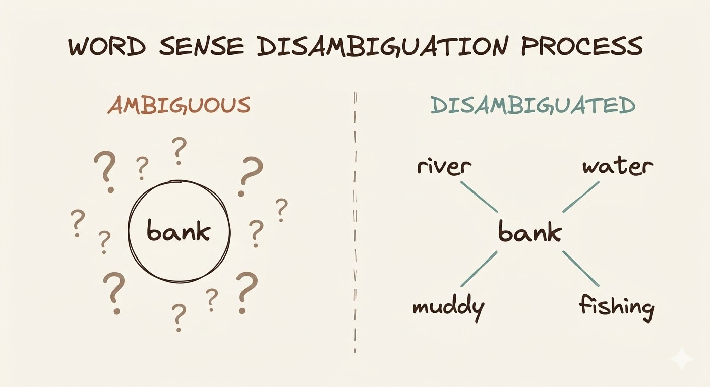
A language model can’t just look at each token independently and hope to build a good summary. It needs tokens to talk to each other, to exchange information, so that each token’s representation gets enriched by its context.

This is the fundamental problem. You have a sequence of token representations. Each one starts out knowing only about itself. You need a mechanism that lets each token selectively absorb information from the other tokens in the sequence.

Enter attention.

The Operation: attention as selective information exchange

Alright, we’ve identified the disease: tokens need context, and they can’t get it by working alone. Time to scrub in. This is the heart of the transformer, and we’re going to open it up properly.

The intuition

Imagine you’re a word in a sentence, and you need to build the best possible representation of yourself. You do this by asking a simple question to every other word in the sequence:

“How relevant are you to me?”

Based on the answer, you take a weighted mix of information from all the other words. Words that are highly relevant to you contribute a lot. Words that are irrelevant contribute almost nothing.

Simple enough. But the devil is in the mechanism that makes this selective exchange learnable. That’s where Query, Key, and Value come in.

Why three projections? The QKV logic

Here’s the part most explanations fumble. They’ll tell you “Q is the query, K is the key, V is the value” and move on, as if naming things explains them. Let’s actually unpack why this decomposition exists.

Consider a medical triage system. When a new patient arrives, three things happen in parallel:

The patient states what they need (the Query): “I have chest pain and I’m short of breath.”

Each specialist posts what they can address (the Key): the cardiologist’s sign says “heart and circulatory issues,” the pulmonologist’s says “respiratory conditions,” the orthopedist’s says “musculoskeletal injuries.”

Each specialist holds their actual expertise and tools (the Value): the cardiologist can run an ECG, interpret troponin levels, and manage arrhythmias. The pulmonologist can read a chest X-ray and manage ventilation. The orthopedist can set fractures.

The triage step is matching the patient’s stated need (Query) against each specialist’s posted capability (Key). The cardiologist and pulmonologist both score high. The orthopedist scores low. The patient then receives a blend of care (Value) weighted by those relevance scores: mostly cardiology and pulmonology, very little orthopedics.

The critical insight: what a specialist advertises (Key) and what they actually deliver (Value) are different things. The Key is a compact, comparable summary optimized for matching. The Value is the full, rich information payload. Separating them lets the model learn what to match on independently from what to transfer. This is what makes attention expressive. If you forced the matching signal and the information payload to live in the same vector, the model would constantly compromise between “being easy to find” and “carrying useful information.”

The same logic applies to why the Query is its own projection rather than just using the raw token embedding. Each token needs to ask a different kind of question than what it is. The word “it” in “The cat sat on the mat. It was warm.” has a specific identity as a pronoun, but its Query needs to express something like “I’m looking for a recently mentioned noun that could be warm.” Those are fundamentally different signals, and they need separate learned transformations to express them.

The math

Now that the intuition is solid, let’s see what this looks like when we write it down. The notation is dense at first glance, but every symbol maps directly to the triage analogy we just walked through.

Given a sequence of n tokens, each represented as a vector of dimension d_model, we stack them into a matrix X of shape (n, d_model).

Three learned weight matrices project each token into the Query, Key, and Value spaces:

\(Q = X @ W_q\)

\(K = X @ W_k\)

\(V = X @ W_v\)

Each output matrix is of shape (n, d_k) while W_Q and W_K have shape (d_model, d_k) and W_V has shape (d_model, d_v). Typically d_k = d_v = d_model / num_heads.

The attention scores are computed by taking the dot product of every Query with every Key:

\(scores = Q @ K^T\)

This produces an n × n matrix where entry (i, j) tells us how much token i should attend to token j. But raw dot products grow in magnitude with the dimension of the vectors, which pushes softmax into regions where its gradients vanish (nearly all the probability mass ends up on a single token). So we scale:

\(scores = (Q @ K^T)/ \sqrt(d_k)\)

The sqrt(d_k) normalization keeps the variance of the scores roughly constant regardless of the dimension, which keeps the softmax in a healthy gradient regime. Think of it as normalizing blood pressure readings by body surface area: the raw number means nothing without accounting for scale.

Then softmax across each row (so each token’s attention weights sum to 1):

\(weights = Softmax(scores)\)

with shape still (n, n).

Finally, each token collects its context by taking a weighted sum of all Value vectors:

\(output = weights @ V\)

which results in a shape (n, d_v).

The full equation, written compactly:

\(Attention(Q, K, V) = Softmax(Q @ K^T / \sqrt(d_k)) @ V\)

In code

Math is nice, but nothing builds confidence like watching the numbers flow. Here’s a minimal, self-contained implementation:

import torch
import torch.nn as nn
import torch.nn.functional as F


class SingleHeadAttention(nn.Module):
    def __init__(self, d_model: int, d_k: int):
        super().__init__()
        self.d_k = d_k
        self.W_Q = nn.Linear(d_model, d_k, bias=False)
        self.W_K = nn.Linear(d_model, d_k, bias=False)
        self.W_V = nn.Linear(d_model, d_k, bias=False)

    def forward(self, x: torch.Tensor) -> torch.Tensor:
        Q = self.W_Q(x)
        K = self.W_K(x)
        V = self.W_V(x)

        scores = Q @ K.transpose(-2, -1) / (self.d_k ** 0.5)
        weights = F.softmax(scores, dim=-1)
        return weights @ V

Let’s check some tensors:

torch.manual_seed(42)

d_model = 8
d_k = 4
seq_len = 4

attn = SingleHeadAttention(d_model, d_k)
x = torch.randn(1, seq_len, d_model)

Q = attn.W_Q(x)
K = attn.W_K(x)
V = attn.W_V(x)

raw_scores = Q @ K.transpose(-2, -1)
print("Raw scores:\n", raw_scores[0].detach())

scaled_scores = raw_scores / (d_k ** 0.5)
print("\nScaled scores:\n", scaled_scores[0].detach())

weights = F.softmax(scaled_scores, dim=-1)
print("\nAttention weights:\n", weights[0].detach())

output = weights @ V
print("\nOutput shape:", output.shape)

The attention weight matrix is the key thing to inspect. If row i has most of its mass in column j, it means token i is drawing most of its contextual information from token j. When people visualize “attention maps” in research papers, this is exactly the matrix they’re showing.

Causal masking: no peeking at the future

Everything we’ve described so far lets every token attend to every other token. That’s fine for tasks like translation, where you have the full input available. But for language generation, there’s a catch: when the model is producing token 5, tokens 6, 7, 8 don’t exist yet. Letting the model attend to them during training would be cheating.

This is enforced by applying a causal mask before the softmax: we set all entries above the diagonal in the score matrix to negative infinity. After softmax, those positions become zero, effectively making them invisible.

def causal_attention(Q, K, V, d_k):
    scores = Q @ K.transpose(-2, -1) / (d_k ** 0.5)
    n = scores.size(-1)
    mask = torch.triu(torch.ones(n, n, dtype=torch.bool), diagonal=1)
    scores = scores.masked_fill(mask, float('-inf'))
    weights = F.softmax(scores, dim=-1)
    return weights @ V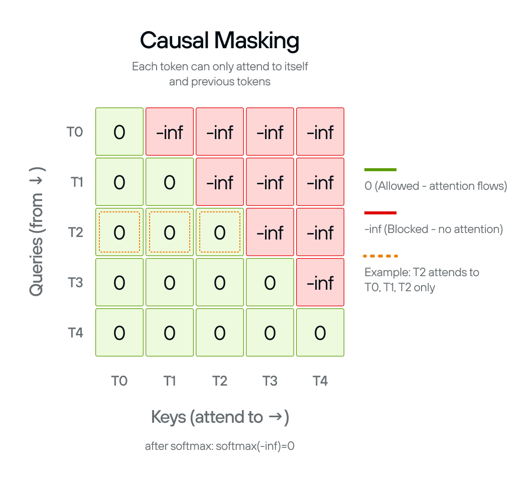

Credits to this article

Multi-head attention: the surgical team

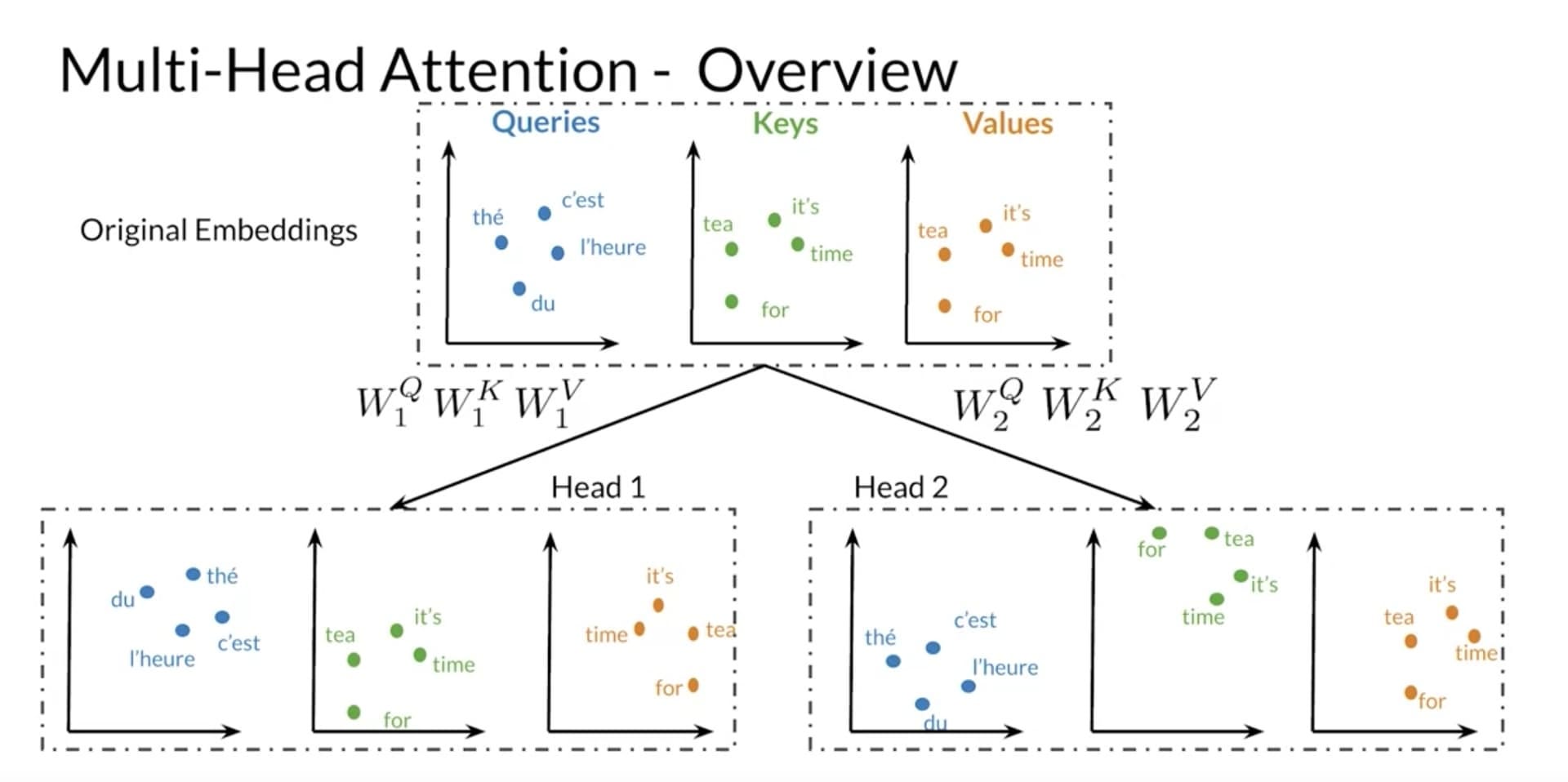
So far we’ve been looking at a single attention operation, one set of Q/K/V projections producing one attention pattern. In practice, that’s a bottleneck. One set of Q/K/V projections can only learn one “type” of relevance. But language has many simultaneous types of relationships: syntactic (subject-verb), coreference (what “it” refers to), semantic (topical similarity), positional (nearby words), and more.

Multi-head attention runs h independent attention heads in parallel, each with its own learned W_Q, W_K, W_V projections. Each head operates on a lower-dimensional slice (d_k = d_model / h), so the total computation is roughly the same as a single head with the full dimension.

Think of it as a surgical team: the cardiologist, the anesthesiologist, and the neurologist all examine the same patient simultaneously. Each looks for different things. Their findings are concatenated and passed through one final linear layer that synthesizes them into a unified assessment.

class MultiHeadAttention(nn.Module):
    def __init__(self, d_model: int, num_heads: int):
        super().__init__()
        assert d_model % num_heads == 0
        self.num_heads = num_heads
        self.d_k = d_model // num_heads

        self.W_Q = nn.Linear(d_model, d_model, bias=False)
        self.W_K = nn.Linear(d_model, d_model, bias=False)
        self.W_V = nn.Linear(d_model, d_model, bias=False)
        self.W_O = nn.Linear(d_model, d_model, bias=False)

    def forward(self, x: torch.Tensor) -> torch.Tensor:
        B, N, D = x.shape

        Q = self.W_Q(x).view(B, N, self.num_heads, self.d_k).transpose(1, 2)
        K = self.W_K(x).view(B, N, self.num_heads, self.d_k).transpose(1, 2)
        V = self.W_V(x).view(B, N, self.num_heads, self.d_k).transpose(1, 2)

        scores = Q @ K.transpose(-2, -1) / (self.d_k ** 0.5)
        weights = F.softmax(scores, dim=-1)
        head_outputs = weights @ V

        concatenated = head_outputs.transpose(1, 2).contiguous().view(B, N, D)
        return self.W_O(concatenated)

The view and transpose operations are just reshaping to split the d_model dimension into (num_heads, d_k) and bring the head dimension forward so all heads compute in parallel via batched matrix multiplication. The final W_O projection mixes the heads’ outputs together. This is where the cardiologist’s ECG findings meet the anesthesiologist’s airway assessment, and the model learns how to combine them.

Credits

What attention actually learns: a practical look

We’ve built the mechanism. But what does it actually do once trained on billions of tokens? It’s worth pausing here, because the patterns that emerge are surprisingly interpretable, and there’s solid research backing this up.

Some heads learn positional attention: they mostly attend to the immediately preceding token, or to the token two positions back. These are the model’s local context sensors. Voita et al. (2019) identified these as one of the three dominant head types in trained translation models, and found that they were among the last to be pruned when compressing the network (Analyzing Multi-Head Self-Attention: Specialized Heads Do the Heavy Lifting, the Rest Can Be Pruned).

Some heads learn syntactic attention: they connect verbs to their subjects across long distances, even through intervening clauses. The sentence “The doctor who treated the patients was tired” requires connecting “was” back to “doctor,” skipping over “patients.” Clark et al. (2019) found that specific BERT heads attend to direct objects of verbs, determiners of nouns, and objects of prepositions with over 75% accuracy, despite never being explicitly trained on syntax (What Does BERT Look At? An Analysis of BERT’s Attention).

Some heads learn rare-token or delimiter attention: they attend strongly to punctuation, sentence boundaries, or special tokens. These act as structural landmarks in the sequence.

Some heads learn induction heads: they implement a simple but powerful pattern-completion algorithm. If the model has seen the pattern “A B ... A” in the context, an induction head will predict that “B” comes next. Olsson et al. (2022) presented evidence that these heads are a key mechanism behind in-context learning, and that they emerge at a specific phase transition during training, coinciding with a measurable bump in the loss curve (In-context Learning and Induction Heads).

None of this is hand-programmed. The Q, K, V weight matrices learn these patterns purely from the training objective of next-token prediction. The architecture provides the capacity for selective information routing; gradient descent discovers which routes are useful.

The Phantom Limb: attention’s missing sense of position

At this point, attention sounds like it solves everything. Tokens can talk to each other, exchange information, build rich contextual representations. But there’s a subtle and critical gap we’ve been glossing over.

Read this:

“The cat sat on the mat. It was warm.”

What does “it” refer to? The cat? The mat? You know the answer partly because of meaning, but also partly because of position. “It” is closer to “mat” in the sequence, and your brain uses that proximity as a cue.

Now here’s the problem: attention, as described above, is completely position-blind. It compares Queries and Keys based purely on what the tokens represent, not where they sit in the sequence. If you shuffled all the words randomly, attention would produce the exact same scores (since each token still has the same Query, Key, and Value content).

For a language model, word order is obviously critical. “Dog bites man” and “Man bites dog” contain the same words but mean very different things.

The fix is simple and elegant: before attention ever runs, you inject positional information directly into each token’s representation. This is called positional encoding.

The original Transformer paper used sine and cosine functions at different frequencies to create a unique positional signature for each position. Modern models use learned positional embeddings (like RoPE) that encode relative distances between tokens rather than absolute positions. The details vary, but the principle is the same: give each token a sense of where it is so that attention can factor in position when deciding relevance.

The Post-Op Summary

We started from the output and traced every component back to the need that created it. The model needs to pick a token, so it needs a good vector. A good vector requires context, so tokens need to exchange information. That exchange is attention: a learnable system of Queries, Keys, and Values that lets each token selectively absorb what’s relevant and ignore what isn’t. Multiple heads run this process in parallel, each specializing in different types of relationships. And because attention on its own has no sense of word order, positional encodings are injected beforehand to give the model a sense of sequence.

Most explanations start with the building blocks and hope you’ll eventually see the big picture. The backwards view forces every component to justify its existence.

That’s the whole architecture, seen from the operating table.